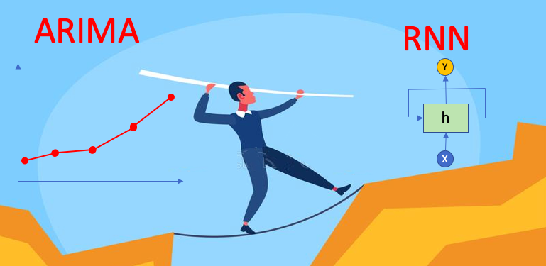
LSTM과 GRU 코드 예시를 찾아 공부하던 중 설명이 가장 자세했던 글을 소개합니다.
설명이 자세해서 ARIMA, RNN, LSTM, GRU 의 차이와 특징을 잘 알 수 있었습니다.
그 중 LSTM과 GRU 를 제가 이해한 바와 함께 정리하겠습니다!
원문
A Technical Guide on RNN/LSTM/GRU for Stock Price Prediction
In our daily lives we interact with chatbot customer services, e-mail spam detections, voice recognition, language translation, or stock…
medium.com
" LSTM 과 GRU 로 주식가격 예측하기 "
1. 데이터 불러오기
1.1. 모듈 불러오기
#!pip install yfinance
import numpy as np
import pandas as pd
import yfinance as yf # Yahoo finance 에서 제공하는 데이터에 접근 가능
yfinance 모듈을 설치하면 야후 파이낸스에서 제공하는 데이터에 접근할 수 있습니다.
1.2. 아마존의 주식 데이터 불러오기
# 아마존의 2013년 부터 2018년까지 일일 주가를 학습 데이터로
# 2019년 데이터를 테스트 데이터로 사용
AMZN = yf.download('AMZN',
start = '2013-01-01',
end = '2019-12-31',
progress = False)
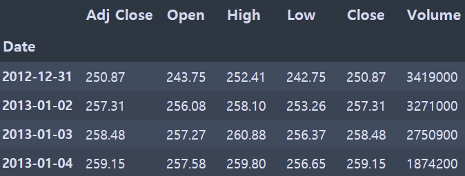
# 수정종가(Adj close), 시가(Open), 최고가(High), 최저가(Low), 종가(Close). 거래량(Volume)
all_data = AMZN[['Adj Close', 'Open', 'High','Low',"Close","Volume"]].round(2)
all_data.head(10)
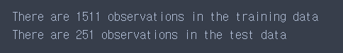
print("There are "+str(all_data[:'2018'].shape[0])+" observations in the training data")
print("There are "+str(all_data['2019':].shape[0])+" observations in the test data")
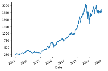
all_data['Adj Close'].plot()2013년 1월 1일부터 2019년 12월 31일까지의 데이터를 불러옵니다.
해당 시기의 수정종가, 시가, 최고가, 최저가, 종가, 거래량을 불러와서 총 X의 변수 개수는 6개가 됩니다.
데이터(all_data)를 살펴보면
print 문 두 가지를 출력하면 training data 행 갯수와 test data 행 갯수를 확인할 수 있습니다.
수정종가(Adj Close)만 가지고 플롯을 그려 데이터의 분포를 시각화해볼 수 있습니다.
2. LSTM / GRU 를 위한 학습데이터 만들기
LSTM 과 GRU로 분석할 때 제가 가장 어려웠던 부분은
(1) 분석이 가능하도록 입력데이터의 구조를 맞추고
(2) 입력데이터의 구조에 맞게 모델 아키텍처를 만드는 일이었습니다.
특히 입력데이터를 이해하는데 꽤 많은 시간이 걸렸어요.
하나 하나씩 뜯어보겠습니다.
2.1. LSTM / GRU 에서 활용하는 입력-출력 구조
LSTM 과 GRU에서는 입력-출력 구조가 다양합니다.
그 중 Many to Many 와 Many to One 이 많이 쓰이게 됩니다.
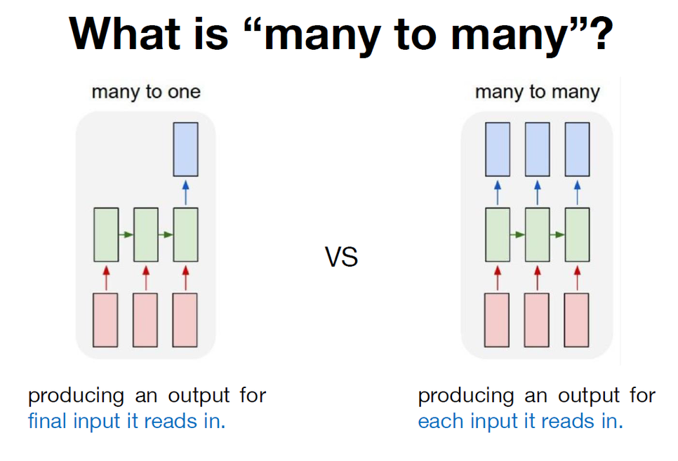
2.1.1. MANY 2 MANY
X가 1차원인 변수로 Many to Many 구조를 만들면 아래와 같습니다.
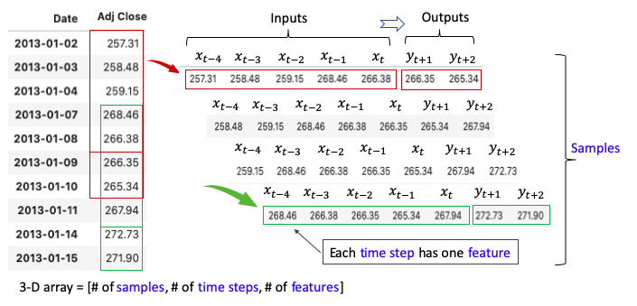
MANY 2 MANY는 과거 X일 동안의 가격을 사용해서 미래 Y일 동안의 가격을 예측합니다.
예를 들어 5일 동안의 가격을 이용해서 미래 2일 동안의 가격을 예측한다고 하면, 아래 그림처럼 빨간색 창(window)을 시리즈에 따라 움직여서 샘플을 만들 수 있습니다.
그러면 각 샘플은 5가지 입력값과 2개의 출력값을 가지게 됩니다.
현재 시점(Xt)으로부터 4일 전까지의 데이터를 입력값으로 사용해 Inputs는 총 5개가 됩니다.
미래의 2일 동안 관측된 y값을 예측하기 때문에 Outputs는 총 2개입니다.
LSTM 과 GRU는 3차원 배열의 입력값을 사용하기 때문에, 데이터를 3차원으로 재구성해줄 필요가 있습니다.
3차원 입력데이터는 ① samples ② time steps ③ features 세 요소로 구성되어 있습니다.
① samples
: 데이터의 크기 (data size라고도 합니다) 이며, 원본 데이터를 window size (위의 그림에서 빨간색 창, 초록색 창의 역할이라고 보시면 됩니다) 에 따라 슬라이싱 할 경우 생기는 데이터의 갯수입니다.
② time steps
: 과거 몇개의 데이터를 볼 것인가를 나타내며, 네트워크에 사용할 시간단위입니다.
③ features
: X의 차원을 의미합니다. 쉽게 말해 X의 변수 갯수입니다.
2.1.2. MANY 2 ONE
이번에는 X가 다차원인 변수를 Many to One 구조로 만들면 아래 그림처럼 됩니다.
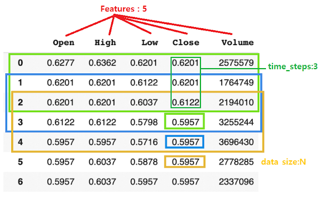
여기서는 현재 시점 데이터와 과거 2일 동안의 가격을 사용해서 미래 1일 동안의 가격을 예측합니다.
5개의 Features를 사용하고 있고
time steps는 3입니다. 만약 원본데이터가 총 7개의 행이라면, window size(features 5개, time steps 3)에 따라 samples(=data size)는 5가 됩니다.
그럼 연속적인(Sequential) 주식가격 데이터는 어떻게 3차원으로 배열될까요?
2.1.3. 3차원 입력데이터
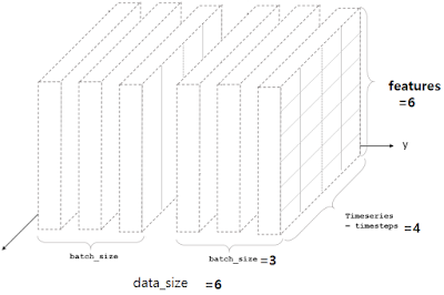
위의 블록은 feature=6, time step=4, sample(=data size)=6 인 데이터를 나타내고 있습니다.
그러니까 연속적인 주식가격 원본 데이터로
- X 변수의 개수 (=features)
- 과거 며칠까지의 값을 반영할 것인가 (=time steps)
- 원본 데이터를 "Features" x "Time steps" 의 형태로 재구성하면 몇 개의 판(?)이 나오는지 (=samples, data size)
파악해서 3 요소를 가진 3차원 블럭으로 만든다는 것입니다.
2.2. 입력값과 출력값 데이터를 위한 코드
def ts_train_test(all_data, time_steps, for_periods):
    """
    input:
     data: 날짜를 인덱스로 가지는 주식가격(Adj Close) 데이터
    output:
     X_train, y_train: 2013/1/1부터 2018-12/31까지의 데이터
     X_test : 2019년 동안의 데이터
    time_steps: # input 데이터의 time steps
    for_periods: # output 데이터의 time steps
    """
    # training & test set 만들기
    ts_train = all_data[:'2018'].iloc[:,0:1].values
    ts_test = all_data['2019':].iloc[:,0:1].values
    ts_train_len = len(ts_train)
    ts_test_len = len(ts_test)

    # training 데이터의 samples 와 time steps로 원본데이터 슬라이싱하기
    X_train = []
    y_train = []
    y_train_stacked = []
    for i in range(time_steps, ts_train_len - 1):
        X_train.append(ts_train[i-time_steps:i,0])
        y_train.append(ts_train[i:i+for_periods,0])
    X_train, y_train = np.array(X_train), np.array(y_train)

    # 3차원으로 재구성하기
    # np.reshape(samples, time steps, features) 로 만듦
    X_train = np.reshape(X_train, (X_train.shape[0], X_train.shape[1],1))

    # Preparing to creat X_test
    inputs = pd.concat((all_data["Adj Close"][:'2018'], all_data["Adj Close"]['2019':]), axis=0).values
    inputs = inputs[len(inputs)-len(ts_test) - time_steps:]
    inputs = inputs.reshape(-1,1)

    X_test = []
    for i in range(time_steps, ts_test_len+ time_steps- for_periods):
        X_test.append(inputs[i-time_steps:i,0])
    X_test = np.array(X_test)
    X_test = np.reshape(X_test, (X_test.shape[0], X_test.shape[1],1))

    return X_train, y_train, X_test
위의 함수에 all_data를 넣고, 5개의 time steps로 미래 2일의 동안을 예측한다고 설정하면(for_periods=2)
X_train은 1505개의 샘플을 가지게 됩니다.
X_train, y_train, X_test = ts_train_test(all_data,5,2)

# 3차원의 X_train을 데이터프레임 형식으로 바꿔서 눈으로 확인해보기
X_train_see = pd.DataFrame(np.reshape(X_train, (X_train.shape[0], X_train.shape[1])))
y_train_see = pd.DataFrame(y_train)
pd.concat([X_train_see, y_train_see], axis = 1)

# 3차원의 X_test를 데이터프레임 형식으로 바꿔서 눈으로 확인해보기
X_test_see = pd.DataFrame(np.reshape(X_test, (X_test.shape[0], X_test.shape[1])))
pd.DataFrame(X_test_see)


print("There are " + str(X_train.shape[0]) + " samples in the training data")
# There are 1505 samples in the training data

print("There are " + str(X_test.shape[0]) + " samples in the test data")
# There are 249 samples in the test data
all_data를 ts_train_test에 넣으면 훈련데이터와 검증데이터가 아래 그림처럼 반환됩니다.
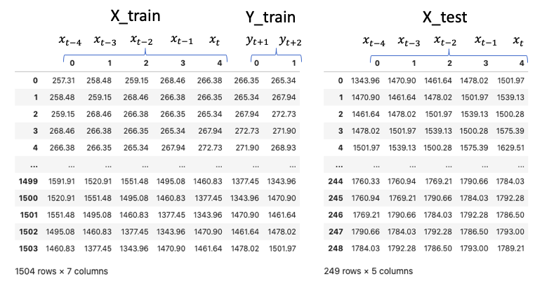
(1504개 행이 아니라 1505개 행일텐데 잘못 나왔나봐요)
2.2.1. 입력 데이터 정규화하기
사실, 몇몇 분석 알고리즘이 그러하듯이
LSTM 과 GRU 는 입력데이터들의 단위가 다른데 정규화를 하지 않으면 모델이 데이터를 학습하는데 좋지 않을 수 있습니다.
예측을 할 때 단위가 커서 변화값이 큰 데이터에 편향될 수 있기 때문입니다.
그래서 입력데이터를 3차원으로 분리하기 전 정규화 과정을 거치는 것이 일반적입니다.
주의해야할 것은
- 학습데이터만 스케일 변환에 사용한다는 것입니다. (그 후에 테스트 입력 데이터를 변형하기 위해 스케일러가 사용됨)
- X_train과 X_test를 독립적으로 스케일링하면 안 됩니다.
*원문을 그대로 가져오긴 했는데.... 왜 그런지는 아직 공부 중입니다.
2.2.에 있었던 코드에서 # scale the data 부분만 추가하면 입력데이터 정규화를 진행할 수 있습니다.
def ts_train_test(all_data, time_steps, for_periods):
    """
    input:
     data: 날짜를 인덱스로 가지는 주식가격(Adj Close) 데이터
    output:
     X_train, y_train: 2013/1/1부터 2018-12/31까지의 데이터
     X_test : 2019년 동안의 데이터
    time_steps: # input 데이터의 time steps
    for_periods: # output 데이터의 time steps
    """
    # training & test set 만들기
    ts_train = all_data[:'2018'].iloc[:,0:1].values
    ts_test = all_data['2019':].iloc[:,0:1].values
    ts_train_len = len(ts_train)
    ts_test_len = len(ts_test)

    # scale the data (데이터 정규화 부분)
    from sklearn.preprocessing import MinMaxScaler
    sc = MinMaxScaler(feature_range=(0,1))
    ts_train_scaled = sc.fit_transform(ts_train)

    # training 데이터의 samples 와 time steps로 원본데이터 슬라이싱하기
    X_train = []
    y_train = []
    y_train_stacked = []
    for i in range(time_steps, ts_train_len - 1):
        X_train.append(ts_train[i-time_steps:i,0])
        y_train.append(ts_train[i:i+for_periods,0])
    X_train, y_train = np.array(X_train), np.array(y_train)

    # 3차원으로 재구성하기
    # np.reshape(samples, time steps, features) 로 만듦
    X_train = np.reshape(X_train, (X_train.shape[0], X_train.shape[1],1))

    # Preparing to creat X_test
    inputs = pd.concat((all_data["Adj Close"][:'2018'], all_data["Adj Close"]['2019':]), axis=0).values
    inputs = inputs[len(inputs)-len(ts_test) - time_steps:]
    inputs = inputs.reshape(-1,1)

    X_test = []
    for i in range(time_steps, ts_test_len+ time_steps- for_periods):
        X_test.append(inputs[i-time_steps:i,0])
    X_test = np.array(X_test)
    X_test = np.reshape(X_test, (X_test.shape[0], X_test.shape[1],1))

    return X_train, y_train, X_test
함수에 데이터, time steps, for_periods 넣어서 X_train, y_train, X_test, sc 반환하기 ↓↓
X_train, y_train, X_test, sc = ts_train_test_normalize(all_data, 5,2)
3. LSTM 모델 코드
def LSTM_model(X_train, y_train, X_test, sc):
    # 필요한 모듈 불러오기
    from keras.models import Sequential
    from keras.layers import Dense, SimpleRNN, GRU, LSTM
    from keras.optimizers import SGD

    # LSTM 아키텍처 (architecture)
    my_LSTM_model = Sequential()
    my_LSTM_model.add(LSTM(units = 50,
                           return_sequences = True,
                           input_shape = (X_train.shape[1],1),
                           activation = 'tanh'))
    my_LSTM_model.add(LSTM(units = 50, activation = 'tanh'))
    my_LSTM_model.add(Dense(units=2))

    # 컴파일링 (Compiling)
    my_LSTM_model.compile(optimizer = SGD(lr = 0.01, decay = 1e-7,
                                         momentum = 0.9, nesterov = False),
                         loss = 'mean_squared_error')

    # training data 세트에 피팅하기 (fitting)
    my_LSTM_model.fit(X_train, y_train, epochs = 50, batch_size = 150, verbose = 0)


    # X_test를 LSTM 모델에 넣어서 예측하기
    LSTM_prediction = my_LSTM_model.predict(X_test)


    # 스케일러에 예측값 넣어 반환하기
    LSTM_prediction = sc.inverse_transform(LSTM_prediction)

    return my_LSTM_model, LSTM_prediction
LSTM 모델을 구축하는 데 필요한 요소는 세 가지입니다.
① 아키텍처 ② 컴파일링 ③ 피팅
① 아키텍처
: LSTM 의 모델을 어떤 구조로 쌓을 것인지 정하는 부분
즉, 모델을 이런 구조로 만들었어~! 하는 것
▶ model = Sequential()
Sequential 모델은 레이어를 선형으로 연결하여 구성합니다.
레이어 인스턴스를 생성자에게 넘겨줌으로써 Sequential 모델을 구성할 수 있습니다.
여기에 .add( ) 메소드로 레이어를 추가할 수 있습니다.
모델은 입력 정보를 필요로 하기 때문에 Sequential( ) 모델의 첫 번째 레이어는 입력 형태에 대한 정보를 받습니다.
두 번째 이후 레이어들은 자동으로 형태를 추정할 수 있기 때문에 형태 정보를 가질 필요는 없습니다.
▶ model.add(LSTM( ))
input_shape 인자를 첫 번째 레이어에 전달 (input_shape 에 배치차원 batch dimension 은 포함되지 않음)
하..... 안에 들어가는 요소들은 정말 뭐가 많네요ㅎㅎㅎ 한 번에 정리하기는 어려워서 일단 텐서플로 링크에 자세한 설명!
tf.keras.layers.LSTM | TensorFlow Core v2.5.0
Long Short-Term Memory layer - Hochreiter 1997.
www.tensorflow.org
▶ model.add(Dense( ))
모든 입력 뉴런과 출력 뉴런을 연결하는 전결합층
오오.... 딥러닝 모델 구축을 블럭 쌓기로 설명하는 좋은 블로그에서 Dense 에 대한 설명을 긁어왔습니다!!
Keras 기본설명 (각 레이어 기능 등)
출처=> https://tykimos.github.io/DeepBrick/ 전체 케라스 세미나 커뮤니티 김태영 둘러보기 | 케라스 코리아 | 캐글 코리아 | RL 코리아 | 최신논문 | 산업AI | DeepBrick for Keras (케라스를 위한..
zereight.tistory.com
② 컴파일링
: 모델을 학습시키기 전에 모델 학습 환경에 대한 설정을 해주는 부분.
즉, 내가 만든 모델을 이런 방식으로 학습시킬거야~! 하는 것
▶ optimizer =
정규화 방법을 지정하는 부분
코드 예시에서는 확률적 경사 하강법(SGD, Stochastic Gradient Descent)을 사용함
※ 확률적경사하강법
- 데이터 1개를 본 후에 loss를 구해서 weight를 업데이트 해주면서 어떤 loss 함수의 진짜 최소값을 찾음
- 전체 train set에 있는 모든 데이터에 1번씩 수행
- 데이터 개수(n번)만큼 update 이루어짐
- "모멘텀" : 관성. weight를 업데이트 할 때 이전에 내려왔던 방향도 반영하자는 개념
- "학습률" : 현재 위치에서 한 걸음에 얼만큼 갈지 결정하는 것
▶ loss =
모델을 최적화시키는데 사용되는 목적함수(= 손실함수)를 지정하는 부분
▶ metric =
분류 문제에서 어떤 것을 기준으로 삼을지 정하는 부분
③ 피팅
: 모델을 학습시키는 부분
즉, 내가 만든 모델을 이런 방식으로 학습시겠다고 한 것을 실행시키는 것
▶ epoch
: one epoch is when an entire dataset is passed forward and backward through the neural network only ONEC
즉, 전체 데이터 셋에 대해 한 번 핛브을 완료한 상태
※ forward pass: 파라미터를 사용해 입력부터 출력까지 각 계층의 weight를 계산하는 과정
※ backward pass: 반대로 거슬러 올라가면서 다시 한 번 계산 과정을 거쳐 기존의 weight를 수정함
이 두 가지를 수행하면서 weight 값을 찾아가는 것을 backpropagation algorithm이라고 함
예를 들어 epoch = 40이라면 전체 데이터를 40번 사용해서 학습을 거치는 것
epoch가 너무 작으면 과소적합, 너무 크면 과대적합의 문제가 있으므로 적절한 epoch 값을 설정해야한다.
▶ batch size
: total number of training examples present in a single batch
즉, 한 번의 batch마다 주는 데이터의 샘플 사이즈
▶ iteration
: the number of passes to complete one epoch
즉, epoch를 나누어서 실행하는 횟수
왜냐하면, 메모리의 한계로 인해 한 번의 epoch에 모든 데이터를 한꺼번에 집어넣을 수 없어서 데이터를 나누어주게 되는데,
몇 번 나누어 주는가 = iteration
각 iteration마다 주는 데이터 사이즈 = batch size
라고 이해하면 됨.
3.1. LSTM 수행한 결과를 플롯으로 그리는 코드
def actual_pred_plot(preds):
"""
Plot the actual vs predition
"""
actual_pred = pd.DataFrame(columns = ['Adj. Close', 'prediction'])
actual_pred['Adj. Close'] = all_data.loc['2019':,'Adj Close'][0:len(preds)]
actual_pred['prediction'] = preds[:,0]
from keras.metrics import MeanSquaredError
m = MeanSquaredError()
m.update_state(np.array(actual_pred['Adj. Close']), np.array(actual_pred['prediction']))
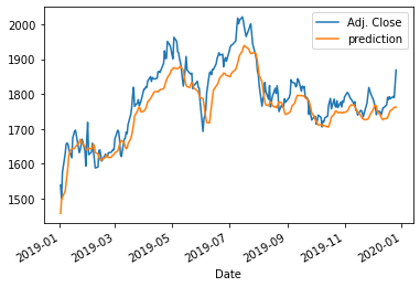
return (m.result().numpy(), actual_pred.plot())실행하기
my_LSTM_model, LSTM_prediction = LSTM_model(X_train, y_train, X_test, sc)플롯 결과
3.2. 예측 성능 지표로 LSTM 수행 결과 확인하기
비교가 가능한 y_pred, y_test 모양으로 구성하기
y_pred = pd.DataFrame(LSTM_prediction[:, 0])
y_test=all_data.loc['2019':,'Adj Close'][0:len(LSTM_prediction)]
y_test.reset_index(drop=True, inplace=True)
예측 성능 출력하는 함수 만들기
(MAE, RMSE, RMSLE, R2 활용)
from sklearn.metrics import mean_absolute_error, mean_squared_error, mean_squared_log_error, r2_score

def confirm_result(y_test, y_pred):
    MAE = mean_absolute_error(y_test, y_pred)
    RMSE = np.sqrt(mean_squared_error(y_test, y_pred))
    MSLE = mean_squared_log_error(y_test, y_pred)
    RMSLE = np.sqrt(mean_squared_log_error(y_test, y_pred))
    R2 = r2_score(y_test, y_pred)

    pd.options.display.float_format = '{:.5f}'.format
    Result = pd.DataFrame(data=[MAE,RMSE, RMSLE, R2],
                         index = ['MAE','RMSE', 'RMSLE', 'R2'],
                         columns=['Results'])
    return Result
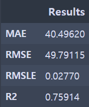
결과 확인 코드
confirm_result(y_test, y_pred)
성능지표 확인 - LSTM
4. GRU 모델 코드
LSTM 과 GRU를 비교하기 위한 것이기 때문에 조건은 LSTM과 일치시켰습니다.
GRU 모델이 LSTM과 차이를 보이는 부분은
GRU에는 (LSTM에는 있는) cell state와 output gate가 없습니다
그래서 LSTM 보다 GRU의 구조가 더 단순합니다
def GRU_model(X_train, y_train, X_test, sc):
    # 모델 만들기
    from keras.models import Sequential
    from keras.layers import Dense, SimpleRNN, GRU
    from keras.optimizers import SGD

    # GRU 아키텍처 (architecture )
    my_GRU_model = Sequential()
    my_GRU_model.add(GRU(units = 50,
                         return_sequences = True,
                         input_shape = (X_train.shape[1],1),
                         activation = 'tanh'))
    my_GRU_model.add(GRU(units = 50,
                         activation = 'tanh'))
    my_GRU_model.add(Dense(units = 2))

    # 컴파일링 (Compiling)
    my_GRU_model.compile(optimizer = SGD(lr = 0.01, decay = 1e-7,
                                         momentum = 0.9, nesterov = False),
                         loss = 'mean_squared_error')

    # 피팅하기 (Fitting)
    my_GRU_model.fit(X_train, y_train, epochs = 50, batch_size = 150, verbose = 0)

    GRU_prediction = my_GRU_model.predict(X_test)
    GRU_prediction = sc.inverse_transform(GRU_prediction)

    return my_GRU_model, GRU_prediction
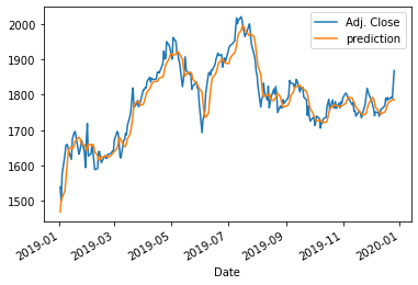
4.1. GRU 결과 플롯 그리기
my_GRU_model, GRU_prediction = GRU_model(X_train, y_train, X_test, sc)
GRU_prediction[1:10]
actual_pred_plot(GRU_prediction)
플롯 결과
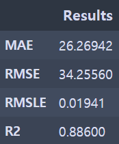
4.2. 예측 성능 지표로 GRU 수행 결과 확인하기
비교가 가능한 y_pred, y_test 모양으로 구성하기
y_pred_gru = pd.DataFrame(GRU_prediction[:, 0])
y_test_gru=all_data.loc['2019':,'Adj Close'][0:len(GRU_prediction)]
y_test_gru.reset_index(drop=True, inplace=True)
결과 확인 코드
confirm_result(y_test_gru, y_pred_gru)
성능지표 확인 - GRU
5. 결론 - LSTM & GRU 비교
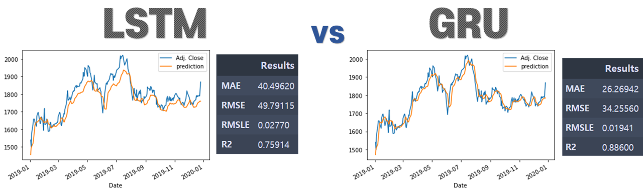
주식가격 예측결과에서는 LSTM 보다 GRU의 성능이 더 좋은 것을 확인할 수 있습니다.
다만 이 과정을 통해 GRU가 꼭 모든 LSTM 모델보다 성능이 좋다고 단정지을 수는 없습니다.
두 모델의 성능은 비슷한 것으로 알려져있고
주제별로 어떤 상황에서는 LSTM 모델이 더 좋기도 하고, 다른 상황에서는 GRU 가 더 좋은 성능을 보이기도 합니다.
그래도 LSTM에 비해 확실한 장점은 GRU는 학습할 가중치의 수가 적다는 것입니다.
※ 전체 소스코드 확인하기 ↓↓↓↓ ※
minji-OH/Analysis_in_Python
Contribute to minji-OH/Analysis_in_Python development by creating an account on GitHub.
github.com
'데이터 분석' 카테고리의 다른 글
| [Pandas/skiprows] 데이터 중간부터 읽어오기 (0) | 2021.07.04 |
|---|---|
| [Pandas/Chunksize] 큰 용량 데이터 읽어오기 (0) | 2021.07.04 |
| [푸리에 변환] 신호 데이터 전처리 - Fast Fourier Transformation (1) | 2021.05.20 |
| [Python/datatable] 용량 큰 csv파일 빠르게 읽기 (0) | 2021.05.20 |
| [의사결정나무] 개념 (0) | 2021.02.22 |


